
Scikit-learn is a powerful Python library widely used for performing complex AI and machine learning (ML) tasks. It is an open-source library that provides numerous robust algorithms, which include regression, classification, dimensionality reduction, and clustering techniques. In this tutorial, we will explore some powerful functions of scikit-learn using scikit-learn toy datasets. Apart from building machine learning models, you will also learn data preprocessing and model evaluation techniques using Python.
Why Do We Use Scikit-Learn?
Scikit-learn is one of Python’s most popular machine learning libraries. The library is enriched with many incredible data preprocessing, model training, and evaluation features. Some of the reasons why AI practitioners prefer scikit-learn are listed below.
Easy to Use
Through scikit-learn, we can quickly implement many basic and advanced statistical and ML techniques. It provides efficient methods that accelerate your workflow with high accuracy.
Detailed Documentation
Scikit-learn provides a comprehensive user guide about supervised and unsupervised algorithms along with many preprocessing techniques. It offers detailed documentation of APIs that learners can easily access.
Widely Used
Due to the advancement in AI and ML, the demand for learning scikit-learn has increased. Scikit-learn dominates the ML market and is extensively used for solving industrial-scale ML problems.
Variety of Optimized Machine Learning Techniques
Scikit-learn majorly covers numerous machine learning algorithms, including classification, regression, clustering, association, and evaluation techniques. In a nutshell, it’s a complete ML package.
Large Community Support
There is a huge community of scikit-learn developers where learners can get advice and direction from experts. According to an estimate, there are around 600,000 monthly scikit-learn users.
Scikit-Learn Datasets
Scikit-learn provides small standard datasets, which we don’t need to download manually. We just need to import it into our code environment (Jupyter notebook) for further use. Using the available toy datasets is a great way to practice various scikit-learn functions. Here is the list of datasets that scikit-learn supports:
- Boston House Prices dataset
- Digits dataset
- Breast Cancer dataset
- Wine Recognition dataset
- Diabetes dataset
- Iris Flower dataset
Important Scikit-Learn Functions
In this tutorial, we will briefly discuss some powerful functions of scikit-learn. You will also learn how to clean data using preprocessing techniques. The tutorial is designed for people who want to kick-start their scikit-learn journey. It will guide you through training various classification models and how to validate them. Regression tasks can be performed using similar code snippets via regression-specific sklearn models. But that is not covered in the scope of this tutorial. Moreover, scikit-learn offers visualization techniques for observing model performance and feature importance. We will also implement them in this tutorial. Let’s begin!
Dataset Exploration
First, you need to install the scikit-learn library in your notebook environment to start using scikit-learn. We can simply install it using the pip command.
#To install the scikit-learn library
pip install scikit-learn
In scikit-learn, we can easily import any dataset into our notebook. First, we need to import the sklearn module, and then we will import the Iris Flower dataset. In the code snippet below, we’ve simply used the load_name() method of the datasets module. For instance, if we want to load an Iris dataset, use load_iris(). You can also import other toy datasets using the same function. The head() command returns the first five rows of the Iris Flower dataset.
import sklearn
from sklearn import datasets
import pandas as pd
data_set= datasets.load_iris()
flower_data = pd.DataFrame(data_set.data, columns=data_set.feature_names)
flower_data.head()
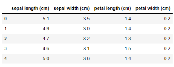
We can also extract the feature names and target variables from the dataset using the feature_names attribute. Here, the features of the Iris Flower are sepal length, sepal width, petal length, and petal width. The target variables are categorized into three classes: Setosa, Versicolor, and Virginica.
target_n = data_set.target_names
feature_nam = data_set.feature_names
print("Feature Names:", feature_nam)
print("Target Names of Iris_dataset:", target_n)

Data Splitting
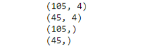
Scikit-learn’s train_test_split() method splits the data into train and test datasets. The training subset is used to fit the model, while the test set evaluates the model’s performance. We’ll split the data into 70% for training and 30% for testing subsets. The method returns four variables: feature matrix for training data (X_traindata), feature matrix for testing data (X_testdata), label array for training data (Y_traindata), and a label array for testing data (Y_testdata). We’ll use the X_traindata.shape command to return the dimensions of the training dataset and X_testdata.shape for testing the dataset.
from sklearn.datasets import load_iris
my_iris = load_iris()
X = my_iris.data
Y = my_iris.target
from sklearn.model_selection import train_test_split
X_traindata, X_testdata, Y_traindata, Y_testdata = train_test_split(
   X, Y, test_size = 0.3, random_state = 1)
print(X_traindata.shape)
print(X_testdata.shape)
print(Y_traindata.shape)
print(Y_testdata.shape)
Applying Classification Algorithms Using Scikit-Learn
Scikit-learn provides numerous classification algorithms, which include k-nearest neighbor, support vector machine, decision tree, random forest, Naive Bayes, linear discriminant analysis, and logistic regression. The complete documentation of how each algorithm works is available on the scikit-learn website. Here we will only discuss k-nearest neighbor, decision tree, logistic regression, and random forest classifier.
K-Nearest Neighbors
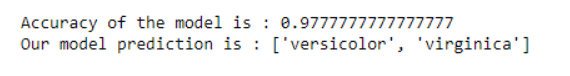
K-nearest neighbors (KNN) is a simple supervised machine learning algorithm. In KNN, we find the similarity between new data (case) and available points using the Euclidean distance formula. To implement the KNN algorithm in scikit-learn, we’ll use the KNeighborsClassifier() function. Here we have used n_neighbors = 3 to find the distance of a new data point from the surrounding three neighbors. The scikit-learn function sklearn.metrics.accuracy_score() is used to find the model’s accuracy on the test dataset, which is around 0.97. Finally, we’ve tested the model’s performance by providing sample data to predict the outcomes.
from sklearn.neighbors import KNeighborsClassifier
from sklearn import metrics
classifier_kNN = KNeighborsClassifier(n_neighbors = 3)
classifier_kNN.fit(X_traindata, Y_traindata)
Y_prediction = classifier_kNN.predict(X_testdata)
print("Accuracy of the model is :", metrics.accuracy_score(Y_testdata, Y_prediction))
#We provide sample data for the prediction of KNN
Dummy_data = [[5, 5, 3,2], [4, 3, 6,3]]
pred_value = classifier_kNN.predict(Dummy_data)
prediction_species =[my_iris.target_names[q] for q in pred_value]
print("Our model prediction is :", prediction_species)
Decision Tree
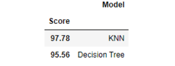
A decision tree is based on rules or conditions. It is a supervised machine learning algorithm used for classification and regression problems. A decision tree has a tree-type hierarchical structure that contains a root node, branches, leaf nodes, and internal nodes. One of the decision tree’s popular variants is called CART. We can easily implement the decision tree using the scikit-learn function DecisionTreeClassifier(). Here, we find the accuracy of the decision tree and k-nearest neighbors through the score() method. The accuracy score of the decision tree is 95%, while the performance score of K-NN is 97%.
from sklearn.tree import DecisionTreeClassifier
decision_tree = DecisionTreeClassifier()
decision_tree.fit(X_traindata, Y_traindata)
Y_prediction = decision_tree.predict(X_testdata)
acc_decision_tree = round(decision_tree.score(X_testdata, Y_testdata) * 100, 2)
knn = KNeighborsClassifier(n_neighbors = 3)
knn.fit(X_traindata, Y_traindata)
Y_pred = knn.predict(X_testdata)
acc_knn = round(knn.score(X_testdata, Y_testdata) * 100, 2)
#To Find the performance of both classifiers
results = pd.DataFrame({
 'Model': [ 'KNN', 'Decision Tree'],
 'Score': [ acc_knn, acc_decision_tree]})
result_df = results.sort_values(by='Score', ascending=False)
result_df = result_df.set_index('Score')
result_df
Decision Tree with K-Fold Cross Validation
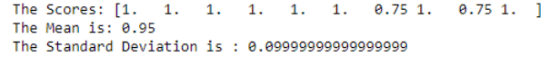
The k-fold cross-validation method gives a generalized model with better accuracy. In scikit-learn, cross-validation can be implemented using the cross_val_score() function. The default value is set at k=10, so it completes ten iterations, and for every iteration, it takes a random distribution of training and testing datasets. For output, it gives the mean accuracy of all folds and the standard deviation (SD) value, which shows the deviation of scores in each fold.
from sklearn.model_selection import cross_val_score
random_f= DecisionTreeClassifier(max_depth=8)
The_scores= cross_val_score(random_f, X_testdata,Y_testdata,cv=10,scoring ="accuracy")
print("The Scores:", The_scores)
print("The Mean is:", The_scores.mean())
print("The Standard Deviation is :", The_scores.std())
Random Forest Classifier
A random forest classifier is a collection of decision trees. Using bagging and feature randomness, it builds each tree and creates an uncorrelated forest of trees, which has better prediction than an individual tree. Ensemble learning is used in the random forest classifier, in which multiple classifiers sort out a complex problem and improve the model’s performance. The scikit-learn RandomForestClassifier() method is used to implement the random forest classifier. It takes the number of trees and maximum features as parameters. Here, the random forest classifier’s accuracy is 0.95 for the Iris Flower dataset.
from sklearn.ensemble import RandomForestClassifier
number_trees = 100
maximum_features = 4
my_model= RandomForestClassifier(n_estimators=number_trees,max_features=maximum_features)
my_model.fit(X_traindata,Y_traindata)
y_predict=my_model.predict(X_testdata)
print("Accuracy of model:",metrics.accuracy_score(Y_testdata, y_predict))

Evaluation Metrics for Classification Algorithms
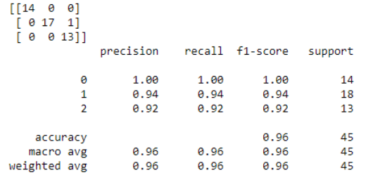
The performance of the model can be evaluated using a confusion matrix and classification report, which includes the model’s recall, f1 score, and precision metrics. A confusion matrix is a summary matrix of the prediction outcomes in a classification problem. It shows the number of true and false predictions made by your classifier. The confusion matrix shows how our model is confused when it predicts the outcomes. It also tells us which type of error (type-1/type-2) is made by our classifier to predict the results. The confusion matrix checks the model’s true positive and negative results. The classification report is another evaluation matrix to measure the performance of your classification model. It shows the value of precision, recall, f1 score, and support. Here we’ll mainly focus on implementing these evaluation metrics using scikit-learn. We have calculated the confusion matrix and classification report for our trained Logistic Regression model. First, we need to import the Logistic Regression classifier. Then we import the confusion matrix and classification report using scikit-learn functions. The result shows the outcomes for the Iris Flower dataset. On the diagonal of a 3 x 3 confusion matrix, we have the true positive values, which means our model has truly predicted the results. The performance of our classifier, in this case, is highly accurate, which can be observed from the classification report.
from sklearn.linear_model import LogisticRegression
from sklearn.metrics import confusion_matrix
from sklearn.metrics import classification_report
log_regression = LogisticRegression()
log_regression.fit(X_traindata, Y_traindata)
Y_predict_val = log_regression.predict(X_testdata)
confusion_mat = confusion_matrix(Y_testdata, Y_predict_val)
print(confusion_mat)
print(classification_report(Y_testdata, Y_prediction))
Data Preprocessing Techniques
The scikit-learn module sklearn.preprocessing provides many data preprocessing techniques. These techniques help clean raw data before model training. This section will explore preprocessing techniques like binarization, standardization, and min-max normalization.
Binarization
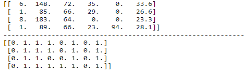
Binarization divides raw data into two categories and assigns values to them using a threshold. If the values are much less than the threshold, then assign 0 to all the values; otherwise, 1. In the code snippet below, we’ve used scikit-learn’s Binarizer() method and kept the threshold=7. Values below 7 are converted into 0, while values above 7 are transformed into 1.
import pandas as pd
import numpy as np
from sklearn.preprocessing import Binarizer
my_URL ='https://raw.githubusercontent.com/andrewgurung/data-repository/master/pima-indians-diabetes.data.csv'
my_columns=['preg', 'plas', 'pres', 'skin', 'test', 'mass', 'pedi', 'age', 'class']
my_data= pd.read_csv(my_URL, names =my_columns)
myraw_data = my_data.values
my_X = myraw_data[:, 0:6]
my_Y = myraw_data[:, 7]
Apply_binarizer = Binarizer(threshold=7.0).fit(my_X)
np.set_printoptions(6)
print(my_X[:4,])
print('-'*60)
print(binaryX[:4,])
Min Max Scaling
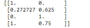
Another data preprocessing method is MinMaxScaler(), which transforms data into 0 and 1. This method is used to smooth the raw data.
from sklearn.preprocessing import MinMaxScaler
Dummy_data = [[11, 2], [3, 7], [0, 10], [11, 8]]
my_scaler = MinMaxScaler()
model=scaler.fit(Dummy_data)
min_maxdata=model.transform(Dummy_data)
print(min_maxdata)
The scikit-learn function preprocessing.scale() standardizes the data along any axis. By default, the axis value is 0, which means standardizing each feature of the dataset.
data_standardized = preprocessing.scale(flower_data)
print("Mean of standardized data: ",data_standardized.mean(axis=0))
print("SD of standardized data: ",data_standardized.std(axis=0))
Visualizing Model Performance & Feature Importance
This section will discuss two important graphs in scikit-learn: the AUC-ROC curve and feature importance.
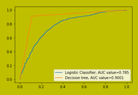
AUC-ROC
With the ROC graph, we can compare the performance of two models: it gives results based on the true positive and true negative predictions. The ROC value is measured from 0 to 1, with 1 representing highly accurate predictions made by the model. Here we have compared the ROC values of logistic regression and decision tree classifiers on sample data.
#make a sample dataset
X,y = datasets.make_classification(n_samples=5000,
                                    n_features=4,
                                    n_informative=3,
                                    n_redundant=1,
                                    random_state=0)
#split the dataset into training and testing sets
X_training, X_testing, y_training, y_testing = train_test_split(X, y, test_size=.3,random_state=0)
plt.figure(0).clf()
#fit logistic regression model and plot ROC curve
model = LogisticRegression()
model.fit(X_training, y_training)
my_predict = model.predict_proba(X_testing)[:, 1]
fpr, tpr, _ = metrics.roc_curve(y_testing, my_predict)
my_auc = round(metrics.roc_auc_score(y_testing, my_predict), 4)
plt.plot(fpr,tpr,label="Logistic Classifier, AUC value="+str(my_auc))
#fit gradient boosted model and plot ROC curve
from sklearn.tree import DecisionTreeClassifier
decision_tree = DecisionTreeClassifier()
decision_tree.fit(X_training, y_training)
my_predict = decision_tree.predict_proba(X_testing)[:, 1]
fpr, tpr, _ = metrics.roc_curve(y_testing, my_predict)
my_auc = round(metrics.roc_auc_score(y_testing, my_predict), 4)
plt.plot(fpr,tpr,label="Decision tree, AUC value="+str(my_auc))
plt.legend()
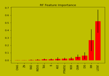
Feature Importance
The feature importance graph shows how important a feature is to predict the target variable. With scikit-learn, we can easily find the feature importance graph using skplt.estimators.plot_feature_importances() of each model. To draw this graph, we’ve considered the Boston dataset using a random forest regressor to figure out which feature contributes more to predicting the outcomes.
import scikitplot as skplt
import sklearn
from sklearn.datasets import load_boston
from sklearn.model_selection import train_test_split
from sklearn.ensemble import RandomForestClassifier, RandomForestRegressor
import matplotlib.pyplot as plt
data_boston = load_boston()
X_data, Y_data = boston.data, boston.target
print("The sample Size: ", X_data.shape, Y_data.shape)
print("The sample size: ", data_boston.feature_names)
X_data_training, X_data_testing, Y_data_training, Y_data_testing = train_test_split(X_data, Y_data,  train_size=0.8, random_state=1)
print("Split data: ",X_boston_train.shape, X_boston_test.shape, Y_boston_train.shape, Y_boston_test.shape)
randomf_reg = RandomForestRegressor()
randomf_reg.fit(X_data_training, Y_data_training)
randomf_reg.score(X_data_testing, Y_data_testing)
fig = plt.figure(figsize=(14,5))
my_axis= fig.add_subplot(121)
skplt.estimators.plot_feature_importances(randomf_reg, feature_names=boston.feature_names,
                                         title="RF Feature Importance",
                                         x_tick_rotation=90, order="ascending",
                                         ax=my_axis);
Wrapping Up
Scikit-learn provides many powerful functions for building and evaluating robust machine learning models. In this tutorial-based article, we’ve explored all the important functions of scikit-learn along with their code samples. Scikit-learn can visualize your model’s performance using the AUC-ROC curve and find important features in a dataset. Due to the wide scope of machine learning, people with good hands-on experience in scikit-learn are in high demand in the job market.
Do you want to dive deep into data science? Make sure to get in touch!