Deep neural networks can be complicated to understand, train and use. Deep learning is still, to a large extent, an experimental science. This is why getting some input on the best practices can be vital in making the most out of the capabilities that neural networks offer. This article presents some good tips and tricks for understanding, training and using deep learning.
1. Distributed representations are essential for deep neural networks
Distributed representations are one of the tricks that can greatly enhance a neural network‘s performance.
The simplest way to represent things with neural networks is to dedicate one neuron to each thing. It’s easy to understand, represent and learn. This is called a localist representation.
However, let’s say you have a classifier that needs to detect people that are male/female, have glasses or don’t have glasses, and are tall/short. With non-distributed representations, you are dealing with 222=8 different classes of people. In order to train an accurate classifier, you need to have enough training data for each of these 8 classes.
In a distributed representation each neuron represents many concepts, and a concept is at the same time represented by many neurons. With distributed representations, each of the properties about an object can be captured by a different dimension. This means that even if your classifier has never encountered tall men with glasses, it would be able to detect them, because it has learned to detect gender, glasses and height independently from all the other examples.
The difference between the localised and the distributed representations is shown in the figures below. In the first figure you can see a localised representation where each neuron learns about one shape.
The figure below shows an example of a distributed representation, where learned properties are shared.
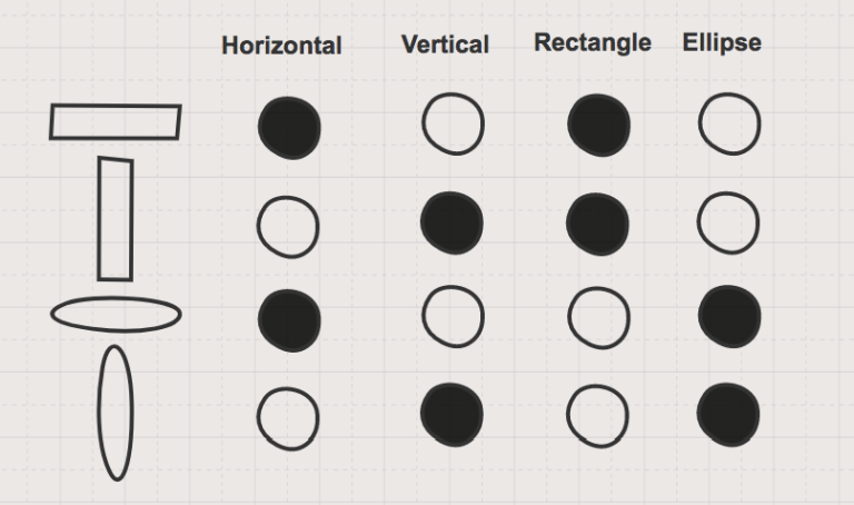
In the figure below you can see how this translates in practice into a description of a circle that also shows how the circle relates to other shapes.

This is the trick that word embeddings (and word2vec) are using, which has given us some very impressive examples.
2. Local minima are not a problem in high dimensions
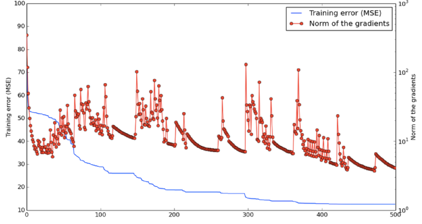
When optimising the parameters of high-dimensional neural nets, there effectively are no local minima. Instead, there are saddle points which are local minima in some dimensions but not all. This means that training can slow down quite a lot in these points, until the network figures out how to escape, but as long as we’re willing to wait long enough then it will find a way. This was experimentally confirmed by Yoshua Bengio’s team.
Below is a graph demonstrating a network during training, oscillating between two states: approaching a saddle point and then escaping it.
Given one specific dimension, there is some small probability that a point is a local minimum, but not a global minimum, in that dimension. While the probability of a point in a 1000-dimensional space being an incorrect local minimum in all of these would be is very small, the probability of it being a local minimum in some of these dimensions is actually quite high. And when we get these minima in many dimensions at once, then training can appear to be stuck until it finds the right direction.
3. Weight initialisation strategy
Xavier initialisation (also called Glorot initialisation) has become some short of standard in deep neural networks. It is implemented in all deep learning frameworks and should be your default weight initialiser.
4. GENERAL DEEP Neural network training tricks
A few practical suggestions from Hugo Larochelle:
- Standardise or normalise real-valued data.
- Decrease the learning rate during training, to avoid overshooting global optima.
- Use momentum, to get through plateaus.
- If you have no clue what parameters to use for training, ADAM can be a good first choice as an optimisation algorithm.
5. Multimodal linguistic regularities
Word embeddings (which were mentioned earlier) are one of the most impressive applications of neural networks. By using word embeddings the neural networks can start understanding the meaning of words.
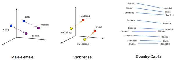
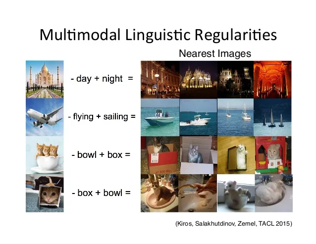
However, the same trick can be used for other concepts. For example, Kiros et al., 2015, demonstrated how this can be used to perform operations on images and words.
6. Minibatches
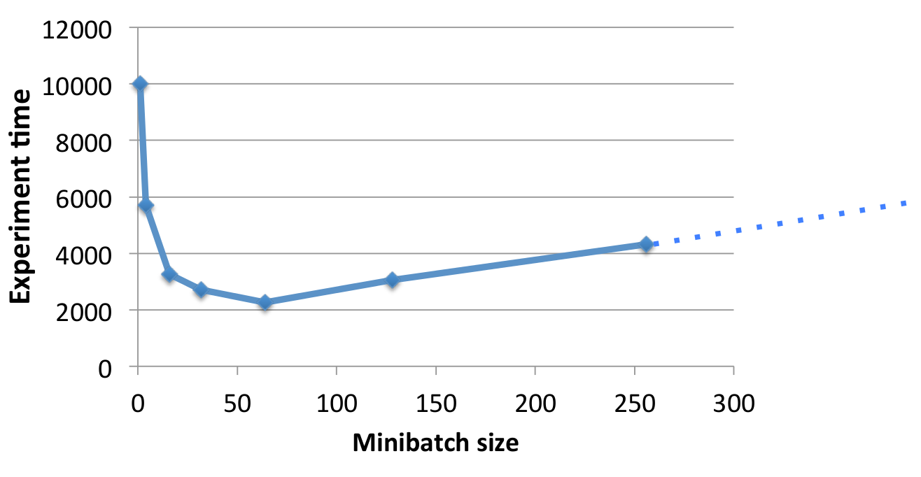
Computing in minibatches can not only improve performance, but it can also improve speed. This avoids some memory operations, and GPUs are great at processing large matrices in parallel.
However, increasing the batch size too much will probably start to hurting the training algorithm and converging can take longer. It’s important to find a good balance in order to get the best results in the least amount of time.
7. Training on adversarial examples
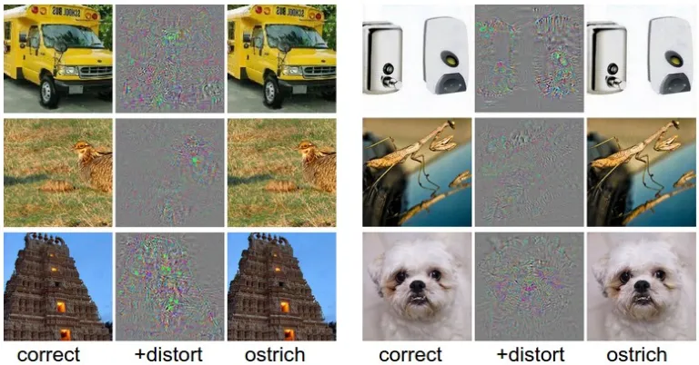
While deep neural networks have given us great success in computer vision, they are not as perfect as it is believed. We can trick neural networks by applying noise which, while impercetible to the human eye, can make them completely misclassify an example. The image is from Andrej Karpathy’s blog post “Breaking Linear Classifiers on ImageNet”, where you can read more about this topic. This is a good reminder that when working with black boxes, we can never be completely sure how the model is operating, and some times we can be met with unexpected bad surprises.
8. Adversarial neural networks
This idea gave rise to the birth of Generative Adversarial Networks. In this framework there are two networks. Neural network D is a discriminative system that aims to classify between real data and artificially generated data. Neural network G is a generative system, that tries to generate artificial data, which D would incorrectly classify as real.
The architecture for this type of network is shown in the figure below.
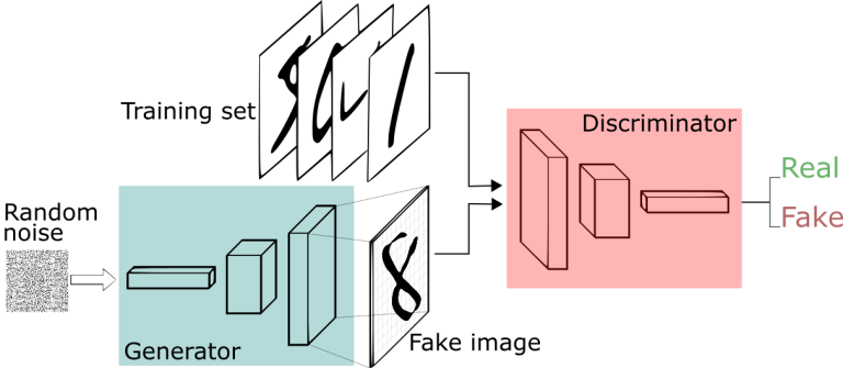
As we train one, the other needs to get better as well. This means two things. First, we get much better discriminators. Secondly, the generators can produce realistic artificial data, such as the fake images of bedrooms you can see below (taken from Radford et al. 2015). Other than the coolness factor, GANs can be used for many other applications such as denoising or aiding human creativity.

9. Optimising gradient updates in neural network training
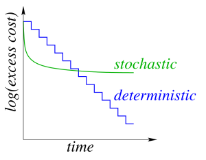
In a deterministic gradient method we calculate the gradient over the whole dataset and then apply the update. The iteration cost is linear with the dataset size.
In stochastic gradient methods we calculate the gradient on one datapoint and then apply the update. The iteration cost is independent of the dataset size.
Each iteration of the stochastic gradient descent is much faster, but it usually takes many more iterations to train the network, as this graph illustrates:
In order to get the best of both worlds, we can use batching. More specifically, we could do one pass of the dataset with stochastic gradient descent, in order to quickly get on the right track, and then start increasing the batch size. The gradient error decreases as the batch size increases, although eventually the iteration cost will become dependent on the dataset size again.
Interested to learn more about neural networks? Make sure to check some of my videos below:

