In the field of machine learning, the evaluation of classification model performance is a critical aspect. Lift, a well-regarded metric, plays an essential role in this evaluation, especially in contexts such as targeted marketing and fraud detection. This article aims to provide a detailed overview of calculating and interpreting Lift and its implementation using Python within a machine learning framework.
Building a Predictive Model
The process to calculate Lift begins with the development of a predictive model. Specifically, a binary classification model is trained using historical data to discriminate between two classes effectively. This model predicts the probability of each instance belonging to the positive class.
Steps to Calculate Lift
1. Model Training and Prediction
A binary classification model, such as logistic regression or a random forest classifier, is trained on historical dataset. The model is then used to predict the probabilities of the positive class for each instance in the dataset. You can easily find models like these in Scikit-Learn.
2. Ranking Instances
All instances in the dataset are sorted in descending order based on the predicted probabilities of being in the positive class.
3. Dividing Instances into Bins
The sorted instances are divided into equal-sized bins. Each bin contains instances with similar predicted probabilities, facilitating a more detailed analysis of the model’s performance.
4. Baseline Calculation
A baseline is established by calculating the number of positive responses expected through random selection.
5. Model Performance Calculation
The number of positive responses in each bin, as predicted by the model, is calculated.
6. Lift Calculation
Lift for each bin is calculated by dividing the model’s performance (the number of positive responses) by the baseline performance. A popular way to do this is to divide the cumulative number of predicted positives to the actual number of predicted positives.
cumsum(predicted_positives)/cumsum(actual_positives)Visualizing Lift with a Lift Curve
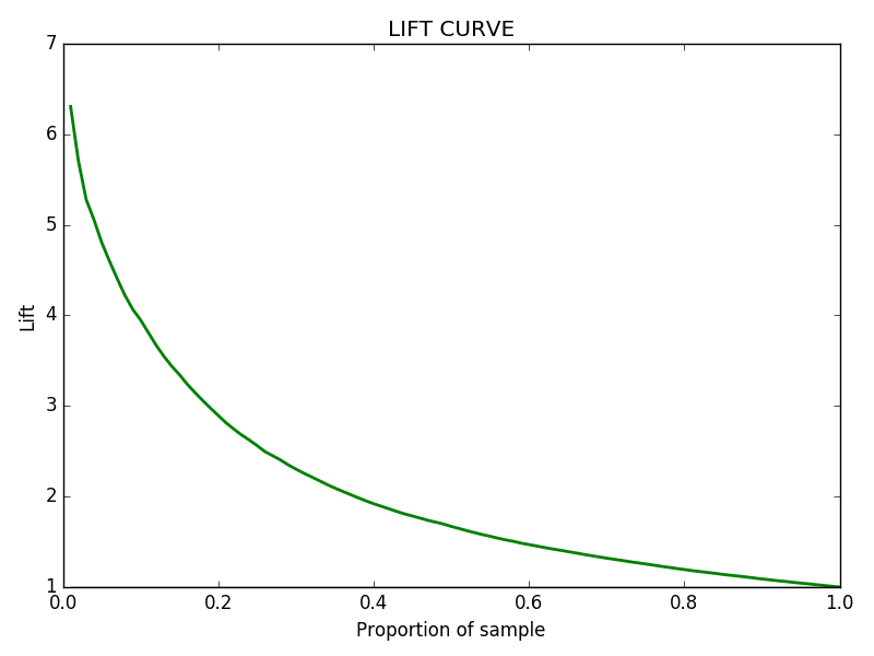
A Lift curve is plotted with the bins on the X-axis and the calculated Lift on the Y-axis. A higher Lift value indicates that the model is effective in identifying positive instances compared to random selection.
For instance, if the baseline positive response rate is 5% and the model identifies a bin with a 20% positive response rate, the Lift is 4.0. This quantitatively shows that using the model is four times more effective than random selection in identifying positive instances.
Implementing Lift Calculation in Python
Below is a Python example utilizing a random forest classifier for model training, prediction, and Lift calculation.
If you run this successfully you should get the following curve:
import pandas as pd
import numpy as np
import matplotlib.pyplot as plt
from sklearn.model_selection import train_test_split
from sklearn.ensemble import RandomForestClassifier
from sklearn.datasets import load_breast_cancer
import pandas as pd
import numpy as np
import matplotlib.pyplot as plt
from sklearn.model_selection import train_test_split
from sklearn.ensemble import RandomForestClassifier
from sklearn.datasets import load_breast_cancer
# Loading the breast cancer dataset
data = load_breast_cancer()
X = pd.DataFrame(data.data, columns=data.feature_names)
y = pd.Series(data.target)
# Splitting the dataset into training and testing sets
X_train, X_test, y_train, y_test = train_test_split(X, y, test_size=0.2, random_state=42)
# Training the random forest classifier
model = RandomForestClassifier(500,random_state=42)
model.fit(X_train, y_train)
# Predicting probabilities of the positive class
probabilities = model.predict_proba(X_test)[:, 1]
# Creating a DataFrame for probabilities and actual target values
df = pd.DataFrame({'probability': probabilities, 'target': y_test})
# Sorting instances by predicted probabilities in descending order
df = df.sort_values(by='probability', ascending=False)
# Adding a column of predicted positive based on a threshold of 0.5
df['predicted_positive'] = (df['probability'] >= 0.5).astype(int)
# Dividing instances into deciles
df['decile'] = pd.qcut(df['probability'], q=10, labels=False, duplicates='drop')
# Calculating the cumulative number of expected positives based on model decisions
df['cumulative_expected_positives'] = df['predicted_positive'].cumsum()
# Calculating the cumulative number of actual positives
df['cumulative_actual_positives'] = df['target'].cumsum()
# Getting the final lift value for each decile
final_lift_per_decile = df.groupby('decile')['cumulative_expected_positives'].sum()/df.groupby('decile')['cumulative_actual_positives'].sum()
# Print the lift values for each decile
print("Lift values for each decile:")
print(final_lift_per_decile)
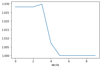
#plotting the lift curve
final_lift_per_decile.plot()Conclusion
Lift is a significant metric in evaluating the performance of binary classification models. It offers a quantitative means to measure how effectively a model identifies positive instances compared to a baseline of random selection.
In applications such as targeted marketing and fraud detection, where prioritizing predictions is crucial, Lift serves as an instrumental tool for informed decision-making.
It is always essential to tailor the interpretation of Lift according to the specific context and objectives of each application and dataset.